TLDR
picoLLM Compression is a novel large language model (LLM) quantization algorithm developed within Picovoice. Given a task-specific cost function, picoLLM Compression automatically learns the optimal bit allocation strategy across and within LLM's weights. Existing techniques require a fixed bit allocation scheme, which is subpar.
picoLLM Compression comes with picoLLM Inference Engine, which runs on CPU and GPU across Linux, macOS, Windows, Raspberry Pi, Android, iOS, Chrome, Safari, Edge, and Firefox. The picoLLM Inference Engine supports open-weight models, including Gemma, Llama, Mistral, Mixtral, and Phi.
We present a comprehensive open-source benchmark results supporting the effectiveness of picoLLM Compression across different LLM architectures. For example, when applied to Llama-3-8b [1], picoLLM Compression recovers MMLU [2] score degradation of widely adopted GPTQ [3] by 91%, 99%, and 100% at 2, 3, and 4-bit settings. The figure below depicts the MMLU comparison between picoLLM and GPTQ for Llama-3-8b.
Why Bother?
LLMs are becoming the de facto solution for any problem! The underlying Transformer architecture has proven highly effective, and throwing billions of free parameters at it enabled functionalities deemed sci-fi beforehand. The growth of model sizes from millions to billions comes with footnotes; LLMs require vast specialized computing and memory resources. So far, this problem has been remedied using the newest and greatest products pushed out by NVIDIA and alike. However, this strategy is not financially sustainable. Also, enterprises become vulnerable as their data needs to travel to third-party data centers. LLMs must run at a much lower cost and where the data resides. i.e., end user's device, on-premises, and private cloud.
LLM quantization can help in two ways. First, by shrinking the model, the computing unit (e.g., CPU, GPU, etc.) accesses less RAM per token, which reduces memory access wait time. Second, using compact data types (e.g., int8_t instead of float32_t) enables the usage of Single Instruction Multiple Data (SIMD) instructions so that the compute unit can perform more operations per clock cycle.
SOTA
LLM.int8() [4] is a seminal publication in which the authors identified that direct 8-bit quantization of weights causes significant perplexity degradation unless some salient weights remain in the floating point format. AWQ [5] suggests that the saliency of weights correlates with the magnitude of their activation. SqueezeLLM [6] tries to preserve salient weights by saving them in a sparse floating-point format. GPTQ is arguably the most widely deployed method at the moment. GPTQ fully reconstructs each weight to minimize the quantization error at its output.
Existing methods rely on a fixed bit allocation across the model's weights, which is suboptimal. However, picoLLM learns the optimal allocation as part of the quantization. We observed that the ideal allocation is model and compression ratio-dependent. For example, the three figures below show the optimal distribution of bits across different components of Llama-2-7b [7] at compression ratios of 3, 5, and 7:
Prior quantization techniques have explicit (e.g., LLM.int8() and squeezeLLM) or implicit (e.g., AWQ) thresholds for defining salient weights (i.e., weights that will sit in the first class and are kept intact). Hard thresholding can be suboptimal for two reasons. First, we don't know the optimal value for the threshold, and second, a sharp bipartite separation is not optimal. It is perceivable that the importance of the weights is a continuous spectrum. Hence, our effort to preserve them should follow. We are cheering for the growth of the middle class! picoLLM learns how to distribute bits optimally within a weight. We have observed that such distribution depends on the model and compression ratio. Below are the optimal bit distributions averaged over all weights of Llama-2-7b at compression ratios of 3, 5, and 7:
Are you a software engineer? Learn how picoLLM Inference Engine runs x-bit quantized Transformers on CPU and GPU across Linux, macOS, Windows, iOS, Android, Raspberry Pi, Chrome, Safari, Edge, and Firefox.
Are you a product leader? Learn how picoLLM can empower you to create on-device GenAI features.
Problem Definition
This section presents a formulation that will help derive the algorithm afterward. We present the original model with . We denote the data sequences by where is the sequence index and is the step index within the sequence. In our formulation, the model accepts a set of state tensors at each step :
We use the symbol to denote the model's size:
The goal of quantization is to find another function that closely follows the original:
Such that its size is much smaller than the original model:
This close mapping can be formalized as:
Where for the sake of ease of notation, we introduce the two definitions below:
is a task-specific error function. In prior works, the goal is to keep the final output of the model intact. Normally, this is measured using step-wise perplexity or mean squared error (MSE). However, we can also introduce task-specific error functions. The only constraint on the function is that, given identical outputs, it has to be zero:
Now, in our focus, which is deep learning, we can represent as a linear chain of functions:
Hence, we can have the definition below:
The size of is the summation of sizes of its constituent functions :
Only some of these functions have free parameters. Some can be nonlinearities, such as SILU, GELU, etc. Given the definitions above, we can redefine the original quantization problem formulation as follows. We want to find a set of subfunctions whose collective size is much smaller than the collective size of their counterparts in the original model such that they minimize the cost function:
picoLLM Compression
We present the picoLLM compression algorithm in a top-down manner. First, we discuss inter-functional bit allocation. i.e., how many bits to allocate to each . Then, we focus on finding the optimal subfunction given a size budget.
Inter-Functional Allocation
Assume that given a budget , we already know how to find the ideal . i.e. . Now, the problem is finding the correct allocation among different functions:
The number of weights in an LLM is usually within 100s. Hence, we can learn these using gradient descent or any other optimization algorithm.
Intra-Functional Allocation
In this section, we focus on how to find the optimal subfunction given a cost budget :
is a very rough approximation. Why is it a good approximation? If the output of each layer remains unchanged, then the logits remain unchanged, and hence, the cost function becomes zero. But this is not correct for any non-zero change. Yet, we found it compelling.
Let's assume a subset of subfunctions doesn't have free parameters. We show this set by . We assume that the ideal quantized version of these functions is identical to their unquantized version:
Although this sounds like a sane assumption, it is not strictly mathematically correct.
Now, what remains are the components that have free parameters. Without loss of generality, we assume these are fully connected weights. They can be reformulated as fully connected weights if they are not. We show these using the set . The union of these two subcategories forms all components and that they do not have any intersection .
Hence, finding the optimal subcomponents with free parameters is reduced to finding equivalent (quantized) weights:
The optimal weight condition can be rewritten as:
Where is a valid approximation because a good quantization scheme will keep the output of each subcomponent close to its original; now, we need to massively simplify this condition so that we can find a practical algorithm for solving it. The stream of equations below explains this simplification:
Where is a valid approximation because the point-wise quantization error and the input to the weight are independent variables. Also, the quantization errors for different columns and the inputs at different indices are independent. The independence of inputs is a bit hazy because GPTQ tries to make use of it. In our observations, these inputs, at least, are very much uncorrelated. is a valid approximation because the quantization error is zero-mean.
We adopt the notation to represent a column of the weight. This notation is particularly useful in our discussion:
The size of the weight is the summation of the sizes of its columns:
The problem of finding the ideal quantized weight is the problem of finding ideal quantized columns:
We define the size of the column as:
Hence, the problem can be rewritten as shown below. Which is very similar to the problem we have been trying to solve for inter-function allocation:
The number of columns in an LLM weight is in thousands. Gradient descent or any other approximate solver can effectively learn the allocation of the bits across columns.
Benchmarks
In this section, we present benchmarking results to support the efficacy of the picoLLM Compression algorithm.
Models
Since our goal is to provide a widely applicable compression algorithm, we use six different LLMs in our benchmark:
Algorithms
We compare picoLLM with widely adopted GPTQ. The AutoGPTQ [12] library supports 4-bit, 3-bit, and 2-bit quantization and handles all the LLM models we wish to use in our benchmark. Since picoLLM is an x-bit quantization algorithm, during benchmarks, we set the bit precision for GPTQ, perform the quantization, measure the resulting model's size (safetensors file) in GB, and produce a picoLLM-compressed model of the same size. We set the group_size parameter of the GPTQ algorithm to 128 and damp_percent to 0.1. The GPTQ and picoLLM models both use 128 sequences of 1024 tokens sampled from the train portion of the C4 dataset [13] as the calibration data.
All code and data to reproduce the presented results are available on the LLM Compression Benchmark GitHub repository.
Tasks
MMLU (5-shot)
The figure below shows the MMLU scores of full-precision (float16) and 4-bit, 3-bit, and 2-bit GPTQ and equally-sized picoLLM models.
ARC (0-shot)
The figure below shows the ARC [14] scores of full-precision (float16) and 4-bit, 3-bit, and 2-bit GPTQ and equally-sized picoLLM models.
Perplexity
The figure below shows the Perplexity of full-precision (float16) and 4-bit, 3-bit, and 2-bit GPTQ and equally-sized picoLLM models. The Perplexity is computed on 128 sequences of 1024 tokens sampled from valid portion of C4 dataset.
What's Next?
Start Building
Picovoice is founded and operated by engineers. We love developers who are not afraid to get their hands dirty and are itching to build. picoLLM is 💯 free for open-weight models. We promise never to make you talk to a salesperson or ask for a credit card. We currently support the Gemma 👧, Llama 🦙, Mistral ⛵, Mixtral 🍸, and Phi φ families of LLMs, and support for many more is underway.


